Short Tutorial
download the tutorial package with the datafiles from HERE
Follow the instructions below For users on the DSC linux computer you can run the program using: /research/pbeerli/bin/migrate-n
Tutorial Overview
How to get the TUTORIAL
download the tutorial package with the datafiles from HERE
How to get MIGRATE
you can either use the program that is already installed on the class server /research/pbeerli/bin/migrate-n or install MIGRATE on your own computer from the Migrate download-website. For this tutorial pick the version 4.x (the 3.6 series cannot handle divergence)
Comparison of gene flow models using Bayes Factors with MIGRATE
Most are familiar with the concept of likelihood ratio tests, or Akaike’s Information criterion for model comparison. This tutorial describes how to compare population models using Bayes Factors. These allow comparing nested and un-nested models, without assuming Normality, or large samples. Bayes factors are ratios of marginal likelihoods. In contrast to the maximum likelihood, the marginal likelihood is the integral of the likelihood function over the complete parameter range. MIGRATE can calculate such marginal likelihoods for a particular migration model (Beerli and Palczewski 2010).
Executive Summary
This tutorial steps through all necessary program runs to calculate Bayes factors for comparing different gene flow models. We need to do the following:
- Decide on the models that are interesting for a comparison. The method does not work well for a fishing expedition where one would try to evaluate all possible models; this is only possible only for population models with very few number of populations. It will be possible to enumerate all models for two or three populations but more will be very daunting.
- Run each model through MIGRATE. Use the same prior settings for each of them because the prior distribution has some influence on the Bayes factors. Use the heating menu to allow for at least four chains. The menu supplies a shortcut to specify the temperatures, it is #. It generates temperatures that are spaced in a particular way: they are spaced so that the inverse of the temperature are regularly spaced on the interval 0 to 1. For example, the 4 different chains have temperatures 1.0, 1.5, 3.0, 100,000.0, this results in the spacing 1.0, 0.666, 0.333, and 0.0.
- Compare the marginal likelihood of the different runs and calculate the Bayes factor and calculate the probability for each model.
More Details
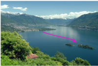
The following pages detail all steps using a small example. We use a simulated dataset that was generated using parameters that force a direction of migration from the population Ascona (A) to the population Brisago (B). The Brissago population is larger than the Ascona population and no individual from Brissago ever goes to Ascona, but Brissago receives about 1 migrant every four generation from Ascona. The dataset name is infile.I (if you are not at the workshop then download here) We will evaluate a total of 3 population models.
- a model with two population sizes and one migration rate to Brissago; both cities exist since a very long time but Brissago is attractive for people in Ascona and they move to Brissago, but not the other way around.
- a model where Ascona is an ancient city and Brissago was built by people who left Ascona some time ago; they became hostile towards each other and nobody moves between the cities.
- a model where Ascona is an ancient city and Brissago was built by people who left Ascona some time ago; Brissago is attractive for people from Ascona and they migrate to there ever since.
. We know the truth therefore we have some prejudice about the ranking of the models, model 3 should be best, models with the same migration pattern as the truth should work better than those with alternative migration patterns, or those with many parameters.
First we need to figure out how to run the dataset efficiently in MIGRATE. For that we pick model 1 and experiment with run conditions until we are satisfied that the run converges and delivers posterior distributions that look acceptable. In practice we would pick the most parameter rich model for this. Here are now the detailed instructions how to rank population genetics models for a particular dataset.
Familiarize with MIGRATE [Tutorial Start]
- Download the tutorial from here HERE and then change into the I directory
- First copy parmfile.I to parmfile_xx0x (in case we need to rerun we keep the original option setting in parmfile.I; the name of the copy reflects the model we use [xx0x see below])
- Start the program: the regular distribution comes in two flavors the single CPU processor version called migrate-n and the parallel processing version that runs on cluster or computers with multiple cores is called migrate-n-mpi. We use a new version of MIGRATE: version 4.2.x. On the cluster you should be able to call /research/pbeerli/bin/migrate-n. (In this text I will call the program from now on simply MIGRATE).
[pbeerli@class-02 migrate_lab]$ migrate-n parmfile_xx0x
On your laptop you may need to use "./migrate-n", if the program is in the same directory. The main menu will appear, looking like this
[pbeerli@class-02 migrate_lab]$ migrate-n parmfile_xx0x

 ++++++++++++++++++++++++++++++++++++++++++++++++++++++++++++++++++
 +                                                                +
 +   POPULATION SIZE, MIGRATION, DIVERGENCE, ASSIGNMENT, HISTORY  +
 +   Bayesian inference using the structured coalescent           +
 +                                                                +
 ++++++++++++++++++++++++++++++++++++++++++++++++++++++++++++++++++
  PDF output enabled [Letter-size]
  Version 4.2.2a   [July-18-2015]
  Program started at   Tue Jul 21 15:03:15 2015


  =============================================================
  MAIN MENU
  =============================================================

  D       Data type currently set to: DNA sequence model
  I       Input/Output formats and Event reporting
  P       Parameters  [start, migration model]
  S       Search strategy
  W       Write a parmfile
  Q       Quit the program


  To change the settings type the letter for the menu to change
  Start the program with typing Yes or Y
===>
- Go to the Input/Output formats menu (press I and hit Enter), in the INPUT section change the Datafile name to infile.I, Return to the main menu by typing Y.
- In the Search strategy menu: Change the Number of recorded steps in chain to 1000, and also change the Burn-in for each chain: to 1000. Do not worry about priors or other runtime options for the moment. Return to the main menu.
- Save the changes by using the menu item Write a parmfile.
- Now run the program (pressing Y will start the run if you are in the main menu).
- The program writes considerable information during the run to the screen, that gives some information about the run. Most interesting are the acceptance ratio for the genealogy and the autocorrelations of the parameter and the genealogy. If the autocorrelation is high and the effective sample size is low (<500) then a longer run may be needed. If the priors boundaries are to tight, then you will see that the values reported are either very close or exactly at the upper prior boundary, in these cases you need to extend the prior range. See prior problems in the output, but for this dataset we will have no such problems.
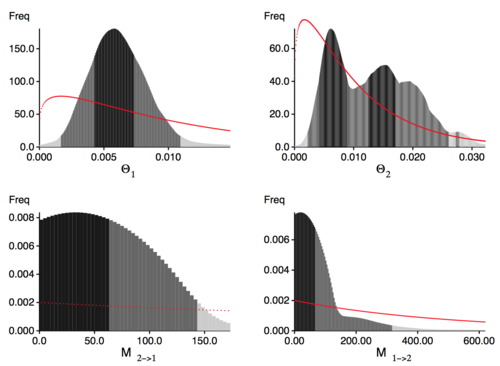
- Look at the outfile.pdf, you will need to transfer the pdf file to your computer and use preview or acrobat or another PDF viewer. In the outputfile look at the figures labeled Bayesian analysis: Posterior distribution, you see histograms similar to the ones in Figure 1. We expect single peaks where the shading of the histogram shows one dark block in the center (50% credibility set), two light gray bars indicating the extent of the 95% credibility set, and two lighter gray bars indication the 99% credibility set. We expect a histrogram that looks smooth that usually has a single peak, commonly similar to an exponential or normal distribution with a heavy right tail.
- In your investigation of Figure 1 you recognize that the histogram has a few kinks because our run was too short. Now restart MIGRATE and set in the strategy menu the setting for change the number of recorded steps in chain from 1,000 to 10,000. This will lengthen the run by a factor of 10.
Because we want to use the thermodynamic integration method for our marginal likelihood calculations, we need to turn on heating. Once again start MIGRATE, use the Strategy menu to turn on heating.
MIGRATE will tell what to do next, you will need to enter 4 chains sampling at every tenth (10) interval using the temperature scheme that is suggested with the character #. Save the parmfile, and run. Here the sequence of entries that you will need to enter:
  ......
  13   Heating:                                                     NO
  16   Run analysis without data:                                   NO

  Are the settings correct?
  (Type Y to go back to the main menu or the number for a menu to change)
===>13
Heating scheme? < NO | YES | STATIC | BOUNDED_ADAPTIVE >
===> Static
Enter the number of different "heated" chains.
Minimum is 4
===> 4
Enter the interval between swapping trees
Enter 0 (zero) for NO swapping
[Current interval is 1]
===> 1
 Enter 4 "temperatures"
[The coldest temperature, which is the first, has to be 1
 For example: 1.0 1.5 3.0 1000000.0]
OR give a range of values  [linear increase:      1 - 10]
                           [exponential increase: 1 @ 10]
or, most lazily, let me suggest a range [simply type a #]
@@@@@ For model comparison, the range of temperatures @@@@@
@@@@@ MUST include a very hot chain (>100000.0)       @@@@@
===> #
Chain         Temperature
-------------------------
   4        1000000.00000
   3              3.00000
   2              1.50000
   1              1.00000

Is this correct? [YES or NO]
===> yes
Don't forget to write the parmfile to save the settings. It should give a better posterior distribution histogram and will add a full table of (natural) log marginal likelihoods is shown towards the end of the outfile_I.pdf, but you may still see double peaks.
With your own data you may want to do another round of refinements, but eventually, by comparing the medians and modes of the parameters in the table and the shape of the histograms you should see a good agreement on similar values, if the modes of the different runs are not within the 50% credibility intervals you certainly need to run longer.
Finally, let's work on the other models
We now start to work on the different models. Remember, we want to run 3 models, and this will take some time, I suggest that you work with your neighbor.
Model 1: xx0x
This model allows migration from Ascona (second population in dataset) to Brissag ( first population in dataset) . The populations are assumed to exist since a very long time. The xx0x in the title is a shortcut for this model; it means that we estimate an immigration rate into the first population and population sizes. I use a particular notion to define the model, read the instructions about the migration/divergence matrix completely before you start typing. Once you have changed the population model,
exit the parameter menu, write the parmfile, run MIGRATE to report follow now the instructions in section Reporting values.
Model 2: xd0x
This model allows divergence, B splits off from A. The second population (A: Ascona) exists for a long time and the population B:Brissago splits off at the time we want to estimate. After that split there is no interaction between the populations. This scenario is equivalent to a species split. The xd0x in the title is a shortcut for this model; it means that we estimate a divergence time and estimate also population sizes. I use a particular notion to define the model, read the instructions about the migration/divergence matrix completely before you start typing. Once you have changed the population model, exit the parameter menu, write the parmfile, run MIGRATE to report follow now the instructions in section Reporting values.
Model 3: xB0x
This model allows divergence, B splits off from A, with migration from A to B after the split. Read the instructions about the migration/divergence matrix completely before you start typing. Once you have changed the population model, exit the parameter menu, write the parmfile, run MIGRATE to report follow now the instructions in section Reporting values.
Report values
We want to compare models, but the tutorial time is too short to do a thorough job and thus our runs will be too short and the posterior distributions of the parameters may still be in bad shape. For our exercise we are mostly interested in the model selection/ordering using marginal likelihoods.
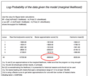
Come to the front and write down the log marginal likelihood into the spreadsheet (look at the example figure labeled Log-Probability of the data given model (marginal likelihood)) [the figure is from a different dataset, so be not alarmed that the marignal likelihoods are different. You will need to report a number from the row labeled All. There are three columns, report the values for the Bezier approximation column.
Migration/Divergence matrix modifications
- Start MIGRATE, choose the Parameter menu.
Choose the entry labeled Model is set to. MIGRATE will now show a dizzying list of options, don't panic, we will only use a few of them. MIGRATE will ask you how many populations are used: enter 2. For a 2-population model we can have 4 parameters. For example, two population sizes and two migration rates. A * or x means that that particular parameter will be unrestrictedly estimated, a zero (0) means that that particular parameter will not be estimated (is not used). Our goal is to set one of the migration/divergence parameters to 0. MIGRATE needs to know how to treat all connections between the populations. The connection matrix is square so we can label it like it is shown in Table 1.
- MIGRATE asks now that you input each row, this can be done by either specifying * 0 (see the lower subtable of Table1) and then return and then entering the next line * * return (second row in second table), or you can enter the whole matrix as * 0 * *.
- For 'Divergence models instead of the '*' you need to enter a 'd' for divergence without migration, and a 'D' for divergence with migration.
| To\From | Brissago | Ascona |
| Brissago | Θ | MA → B |
| Ascona | MB → A | Θ |
| To\From | Brissago | Ascona |
| Brissago | * | * |
| Ascona | 0 | * |
| To\From | Brissago | Ascona |
| Brissago | Θ | ΔA → B |
| Ascona | 0 | Θ |
| To\From | Brissago | Ascona |
| Brissago | * | D |
| Ascona | 0 | * |
Comparing models
How to calculate Bayes factors? In the Table 3 I summarized all log marginal likelihoods, ln(mL), the Bayes factors are often calculated in very different ways. Here, I report the natural log Bayes factors where
Using the guidelines of Kass and Raftery (1995), values smaller than -2 suggest preference for 'model 2', values larger than 2 suggest preference for 'model 1'. We can use the log marginal likelihoods or the BF to order the models (see column Choice in the Table 3).
We also can calculate the model probability. It is calculated by dividing each marginal likelihood by the sum of the marginal likelihoods of all used models:
Note that for the above formula uses the marginal likelihoods, *not* the *log* marginal likelihoods (which is what the program reports). The calculation of model probabilities from the reported log likelihoods is easy with computer programs that have variable precision (for example Maple or Mathematica). Calculations on a desk calculator often fail, for example the likelihood of model 1 is a remarkable small number because the likelihood is exp(-4803.07)= 1.130323625060 x 10-2086, my emulated HP sci 15C calculator delivers 0.0000. But you can calculate the above quantities using this recipe: (1) find the largest log likelihood (-4795.23), (2) subtract that number form each log likelihood in the list (result: -2.27, 0.0, 2.5, -26.67), (3) exponentiate each element in the new list (result: 0.1033, 1.0, 0.0821, 2.6144 x 10⁻¹²) , (4) sum all elements in the list up (0.1033+1.0+0.0821+2.6144 x 10⁻¹²), this is the denominator (1.1854). (5) now divide each element in the list by that sum and the numbers will look like the one in table 3 last column.
I have added a little python script that calculates the model probabilities from the text outfiles: If you want to see the results of the model exercise do:
grep " All " */outfile_* | sort -n -k 4,4 | migbf.py
Table 3: Showing log marginal likelihoods for all models tested (and three more, but without the panmictic model) and model probabilities
Model                   Log(mL)   LBF     Model-probability
-----------------------------------------------------------
1:xxxx:                 -9662.42   -23.73        0.0000
2:xBxx:                 -9661.98   -23.29        0.0000
3:xxBx:                 -9661.52   -22.83        0.0000
4:xd0x:                 -9656.51   -17.82        0.0000
5:xB0x:                 -9649.33   -10.64        0.0000
6:xx0x:                 -9648.93   -10.24        0.0000
7:x0dx:                 -9641.77    -3.08        0.0402
8:x0xx:                 -9641.01    -2.32        0.0859
9:x0Bx: [your model 5]  -9638.69     0.00        0.8739
-----------------------------------------------------------
The MacOS file system is capitalization-blind, D and d are the same,
for that you see capital B which are placeholders for capital D.
Looking at the model probabilities we can see that the “true” model has considerably higher support than the full model or the model that suggests a wrong direction of gene flow.
Summary of results
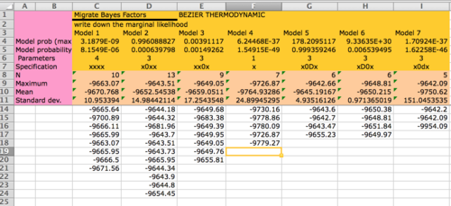
The best model (the one with the highest marginal likelihood) is model 5 (custom-migration={*0D*}). if we use the thermodynamic approximation of marginal likelihood. MIGRATE also reports the harmonic mean, but I suggest to ignore it and use thermodynamic integration (as we did) although it will be more costly to run. It was shown several times (for example, Beerli and Palczewski 2010, Xie et al. 2011 ) that the harmonic mean estimator is not a good estimator and may be misleading and prefer the more complex model. The picture below is a sample from the class tutorial done on August 1st 2011.
References
- Beerli, P. and M. Palczewski. 2010. Unified framework to evaluate panmixia and migration direction among multiple sampling locations. Genetics 185: 313–326.
- Kass, R. E. and A. E. Raftery. Bayes factors. 1995. Journal of the American Statistical Association 90(430): 773– 795.
- Xie, W., P. O. Lewis, Y. Fan, L. Kuo, and M.-H. Chen. 2011 Improving marginal likelihood estimation for Bayesian phylogenetic model selection, Systematic Biology, 60: 150–160.
